Loading video…
All breakouts

103Silent UGCOther hookAI Tools
Hook
you need to nerd out
@chrispathway
25.2K followers · usually 4.6K views a post
Views
462.8K
Likes
83.9K
Comments
219
Shares
2.9K
Why it worked
The post succeeds by curating an aesthetic of high-level intellectual rigor, appealing to students and tech enthusiasts who value the 'nerd' identity and structured learning.
Summary
A student shares a study-with-me style photo dump showing their academic workflow, including math notes, coding projects, and Rubik's cube algorithms. The slides document their progress in statistics, programming, and technical problem-solving.
Structure
- 1Personal introduction at the Eiffel Tower
- 2Display of advanced statistics and linear algebra study notes
- 3Demonstration of an Arduino electronics project
- 4Showcase of a chess game and Chinese checkers
- 5Rubik's cube algorithm notes and practice
- 6Technical coding and data science workflow documentation
On-screen text
you need to nerd out
Done when: you derive the MLE and Fisher information for Bernoulli and Normal unaided.
Week 2—Linear algebra = the regression machine (~16 h)
Intuition: 3Blue1Brown - Essence of Linear Algebra (full series) (3h)
Mechanics: Khan - Linear Algebra - matrix mult, transpose, inverse (A1), rank, identity (4 h)
Quadratic forms, symmetric matrices, positive-definiteness (covariance matrices),
eigenvalues (A2) (3h)
Regression in matrix form: y = Xβ + ε = β = (X'X)⁻¹X'y -> hat matrix H = X(X'X)⁻¹X' -> fitted
values as a projection. ISLR Ch 3 + Fahrmeir et al., Regression (the shared regression reference)
(4 h)
R: vectors, data frames, first 1m() (2h)
Done when: you can write the least-squares solution in matrix form and explain
what the hat matrix does.
Week 3—Distributions bridge + likelihood concepts + R (~16 h)
Distributions toolkit (pmf/pdf, mean, variance): Normal, Bernoulli/Binomial, Poisson,
Exponential, Gamma, Beta. Note the conjugate pairs (Beta-Binomial, Gamma-Poisson, Normal-
Normal) for Bayesian. Blitzstein - targeted (4 h)
Exponential family form (Likelihood part 2 + GLMs) (2 h)
Likelihood machine, run 2: Poisson + Binomial. Then the concepts: standard error, Wald /
score / likelihood-ratio tests, profile likelihood. Primary text below (5 h)
R: 1m() summaries, residual plots, swirl package (3 h)
Review loose ends (2 h)
Done when: you can state pmf/pdf + mean + variance of the main distributions and
recognise a conjugate pair.
Week 4—R fluency + Bayes + consolidate + retest (~16 h)
R for your courses: 1m(), glm(), aov(), reviewing summaries, diagnostics. Meler -
ANOVA and Mixed Models (free, R-based) + R4DS (5 h)
Bayesian by hand: posterior ∝ prior × likelihood, normalizing constant as an integral, a full
Beta-Binomial conjugate update, and the Laplace approximation idea (Taylor around the
mode -> ties back to Week 1) (4 h)
Arduino Tutorial 12: Understanding Potentiometers
Sketch uses 3122 bytes (9%)
Global variables use 200 bytes (9%) of dynar
Tutorial 10
Reading voltage from our
setup:
PinMode(readpin, INPUT);
Serial.begin(9600);
loop:
V2= analogRead(readpin)
Serial.println(V2)
Readvalue between 0
0V
1023
Real voltage = 5/1023 * ReadV
L'U R U' L' U R' R U R' U R U2 R'
U: UPWARD FACE, 90° CW
1 make the daisy
2 white cross
3 solve bottom layer
4 Second layer solved
5 yellow edge piece FUR U'R'F'
-2 yellow edge piece (line, orient towards you: FUR U'R'F'
-2 yellow pieces on line and then FUR U'R'F
5. yellow
6. yellow
-es (rotate until yellow left
R'
F -> R U R' U R U2 R'
L' U R U' L' U R' R U R' U R U2 R'
# Search best set of hyperparameters alpha and p (ONLY RUN THIS ONCE AND THEN SAVE PARAMETERS) -> import numpy as np
# errors in LEVEL space: y_(t+h) - y_hat_(t+h)
errors = actual_s - pred_s
rmse = np.sqrt(np.mean(errors**2))
cv_rmse.append(
"Maturity": target_col,
"Horizon": h,
"alpha": alpha,
"p": p,
"CV_RMSE": rmse,
"H_Forecasts": len(errors)
))
ridge_cv_results = pd.DataFrame(cv_rmse)
ridge_cv_results = ridge_cv_results.set_index(["Maturity", "Horizon"]).sort_index()
print("ridge CV results (by target, evaluated on levels; first rows):")
display(ridge_cv_results.head())
# Choose best (alpha, p) per (Maturity, Horizon)
ridge_best_params = {}
for (mat, h), group in ridge_cv_results.groupby(level=[0, 1]):
best_row = group.sort_values("CV_RMSE").iloc[0]
ridge_best_params[(mat, h)] = {
"p": int(best_row["p"]),
"CV_RMSE": best_row["CV_RMSE"],
"H_Forecasts": int(best_row["H_Forecasts"])
}
print("\nBest Ridge hyperparameters per (Maturity, Horizon) (by target):")
for key, val in ridge_best_params.items():
mat, h = key
print(f"Maturity: {mat}, Horizon: {h} -> alpha={val['alpha']}, p={val['p']},")
print(f" "CV_RMSE={val['CV_RMSE']}, H={val['H_Forecasts']}")
Alpha grid: [0.0, 0.1, 0.15, 0.2, 0.3, 0.4]
Lag grid: [0, 1, 5, 10]
CV for Ridge (by target): target=0052, h=1
(DEBUG RIDGE CV) origin=2014-01-02, train_end_date(h=0)=2013-12-31, max_train_t=2013-12-31, forecast_date(t+h)=2014-01-03
(DEBUG RIDGE CV) origin=2014-01-09, train_end_date(h=0)=2014-01-07, max_train_t=2014-01-07, forecast_date(t+h)=2014-01-10
(DEBUG RIDGE CV) origin=2014-01-16, train_end_date(h=0)=2014-01-14, max_train_t=2014-01-14, forecast_date(t+h)=2014-01-17
4.4.2 Diebold-Mariano Test
ADD HAC ESTIMATOR VARIANCE array; Leybourne, and Newbold (1997). Testing the equality
of prediction mean squared errors, International Journal of Forecasting, 13(2), 281-289. RMSE alone
does not indicate whether differences in forecast performance are statistically meaningful. To test
whether two models achieve the same predictive accuracy, we apply the Diebold-Mariano test as
introduced by Diebold and Mariano (1995). The test compares the squared forecast errors of two
competing models. Let L(e_t+h) = (e_t+h)² denote the loss, and define the loss differential as
d_t+h = L(e_t+h) - L(e_t+h)
The DM statistic is computed as
DM = d_bar / sqrt(V_hat(d_bar) / T)
where d_bar accounts for serial correlation in forecast errors. A significant value indicates that there is a
significant difference in predictive accuracy between the two models (Diebold and Mariano 1995, p.
254).
Original caption
#nerd #math #student #chess #Tech
More from @chrispathway
More breakout videos from this creator.